Power measurement: What sample rate do I need?

Andy Norrie

 

Power measurement: What sample rate do I need?

 

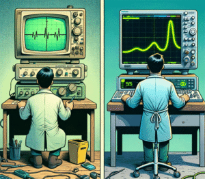
Its very easy to get caught up with how ‘fast’ a scope or power analyser can go, but how important is the sample rate? Is faster always better? Will newer/faster equipment always give you a better result?

Running faster allows us to resolve smaller details and more accurately measure brief spikes. The downsides include a more noisy capture, which can hide the general trend, and a much larger amount of data.

Quarch has been contributing to industry specifications on power measurement, and we thought it would be interesting to look at why certain sample rates are chosen.

 

Sample rate comparison

Let’s start by looking at industry specifications for power measurement. The OCP (Open Compute Platform) among others, specify a ‘moving window average’ for some power measurements. This is used to find the maximum power a device consumes within a workload.

The OCP spec gives two window widths, 100uS and 100mS. In each case, we move the window over the data, averaging each point within the ‘window’, so we give a single value. We look for the window with the highest value, and this is the worst case that we report.

Averaging over a window acts as a filter, reducing the effect of noise and small spikes. It gives a value that is meaningful in terms of the power supply needed for the device.

For a 100mS averaging window, we need to sample multiple times within the 100mS window, but how many times?

 

Introducing our data

For the test, we need something that changes in power consumption a lot over the trace. If the load is steady, almost any sample rate will give the same result, so we need to make a realistic test.

This is a power up capture of a modern enterprise HDD. The full trace is about 12 seconds long and includes a small time with the device off, then the full spin-up sequence until it becomes ready on the host. The trace was captured using our PAM range of power analysis tools and Quarch Power Studio (QPS).

The data was captured at 250 KS/s (4uS between samples) which is the maximum sample rate our device can handle and the rate set in the OCP spec.

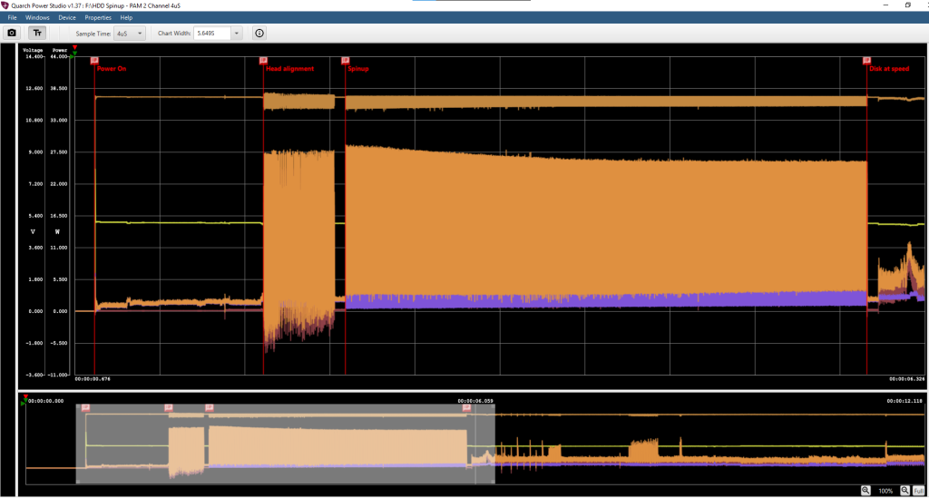
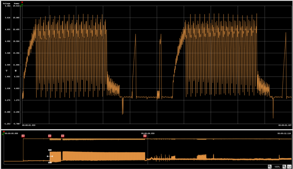
The 12V channel is the one we are interested in, as it drives the motor. During spin-up, the current profile jumps rapidly between several different levels. This means we risk an inaccurate measurement if we do not sample fast enough

 

Processing the data

I used the export feature of QPS to dump the entire trace into a large CSV file of around 275MB.

Next I wrote a quick Python script to remove every second sample from a CSV file. This is a crude but effective way of halving the sample rate. By doing this multiple times, we end up with a set of files, each at half the sample rate of the previous.

This is similar to capturing the spin-up at different sample rates, but has the advantage that we remove the uncertainty that comes from each power-up being different. Here we are working with the same raw data set, which will give a much clearer comparison.

 

OCP 100mS peak power test

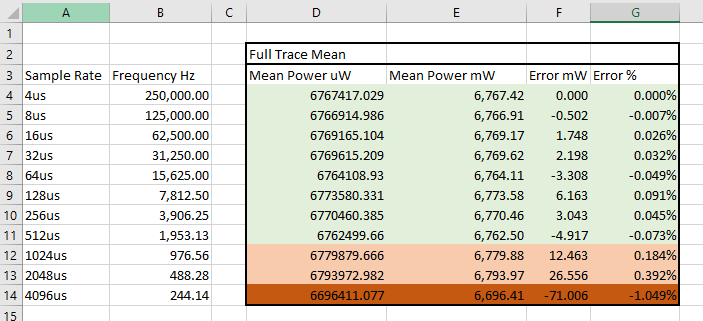
Starting at 4uS sampling (250 KS/s), I worked down to 4096uS (~244 S/s). I then used a second script to run a 100mS averaging window over the data and report the worst case for each sample rate

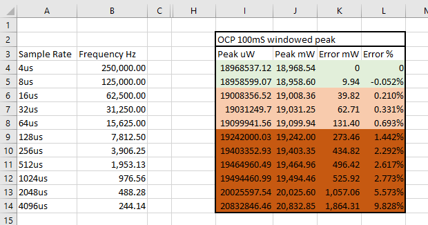
For each sample rate, we have the worst-case (peak) power measured across the 100mS averaging window and can immediately see a problem.

At 4uS and 8uS sampling, there is minimal difference (around 0.05% error), but this rapidly increases and the sample rate drops.

By 128uS sampling (~8 KS/s) we are well over 1% error, and this gets steadily worse. While the magnitude and trend of the error will depend on the data set, this clearly shows that we need at least 10 KS/s if we want to avoid sample rate contributing significantly to the final error. Remember that errors can stack, calibration accuracy, and similar factors have to be accounted for in the total potential error estimate.

 

OCP 100uS peak power test

The OCP test also require a 100uS averaging window. As this is a smaller window, it should follow that we have to sample faster to avoid errors.

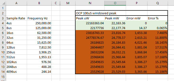
And that turns out to be correct! Again, the 4uS and 8uS sampling rates are very similar, but the errors increase faster with the smaller window. Here, we would not recommend running slower than 125 KS/s to get an accurate result.

The OCP specification requires a base sample rate of 4uS for these measurements, and we can see here that this is a sensible requirement.

 

Workload-average power tests

In other standards, total energy efficiency is the focus, rather than peak power. Here we are more likely to look at the average power over a full workload.

A new standard we are contributing to specifies 4uS sampling, averaged down to 1 sample per second. If a workload takes 100 seconds, then the 100 readings would be further averaged to get the final efficiency result. This allows users to get a basic trend-over-time graph of power usage and also the single average power value for the workload.

Unsurprisingly, we see that taking an average of the whole trace makes for a more stable result as we reduce the sample rate. We effectively have a single ‘window’ that is the size of the whole trace here, and so the error increases more slowly.

In this example, we could have gone as low as ~2KS/s before getting a significant loss of accuracy. This means that the sample rate is important, but not nearly as much as with the peak power tests.

Note that 1 second averaging is NOT the same as 1 second sampling. In the workload averaging test, we will be capturing data at 4uS (250KS/s) and averaging all 250,000 values into a single figure for the second. While this loses detail (as we only have one measurement per second), it perfectly maintains the average power consumption.

Quarch tools always average rather than skip samples, so ensure the most accurate power reading possible.

 

Do we need to go faster?

All the Quarch tools run at 250 KS/s for analog sampling. We saw here that this looked good enough for the above test cases, but that does not prove that we would not see better results at higher rates.

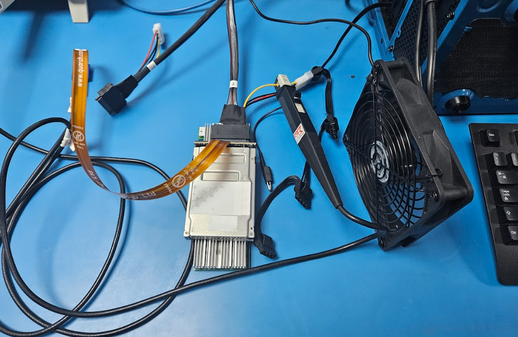
To do this, we grabbed the scope from our lab, which has current probes. This is an older one, but it was a decent unit.

Tektronix DPO 3032 with TCP0030 current probes.

It has a vastly faster sample rate at 2.5 GS/s, though its bandwidth is limited to 300 MHz which makes the higher end less useful.

We hooked up a Gen5 SSD this time to ensure we looked at both drive technologies. We ran the scope at 1 MS/s to. We hooked up the PAM in series so we could capture both tools at the same time.

Let’s zoom in on a small section of the SSD trace and compare at 1 MS/s to 250 KS/s.

We can see that both traces follow the exact same trend; the only difference is that the fast trace has slightly more noise.

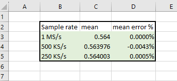
The calculated statistics confirm this; the difference between the 3 sample rates shows extremely small differences to the mean.

This demonstrates that sampling faster than 250 KS/s has no benefit for most tests. By testing both HDD and SDD, we have also ensured our conclusions are accurate for both.

 

Conclusions: 4 costs of speed

When we tried to run the scope comparison in the lab, we quickly hit problems:

This scope has a memory depth of 5 megapoints, so while it can run happily at 50 MS/s, it can only capture at this rate for a fraction of a second. Even at 1MS/s it could not capture the full power-up cycle.

Now our scope is pretty old, but looking at more modern scopes, memory depth is often rather limited.

• • InfiniiVision 4000 X Series Digital Bench Oscilloscope, MSOX4154A

    • $31k USD – 4 Mega points (matching our scope)

• • Keysight DSO91304A Infiniium

    • $41k USD – 1000 Mega points

1. 1. The Keysight 9000 series has a lot of memory, but it has a price to match! Trying to sample at a faster rate than you need can be very costly and yet give no benefit.

   2. A fast ADC sampling rate is of no use unless you are recording and actually using the data from every single sample. If any part of your analysis chain is discarding samples, your effective sample rate is lower.

   3. At high sample rates, the amount of data produced is very significant. A drive generally has 2 power rails, and we need to sample both voltage and current. That is 4 measurement channels and can turn into gigabytes of data quickly at high sample rates.

   4. At high sample rates, you begin to sample increasing levels of ‘noise’ which is not actually part of the true power consumption of the device and can actually make your result less useful. We’ll have more coming on this in a later blog!